Exploring the data - Statistics | Xenia Mountrouidou (DrX)

Graphs are excellent for visual learners. However, sometimes you just need to “show the numbers.” Exploratory Data Analysis (EDA) using statistics offers a compact summary of your data, providing a clear narrative without requiring extensive coding. Thanks to many readily available packages, this process is both accessible and efficient.

In this blog, we will dive into the basics of statistical EDA using Pandas. Along the way, we will revisit key statistical concepts that challenge assumptions about your data. The accompanying code can be found in the notebook blog_eda_2.ipynb.

1,000 ft view

What?

Statistical analysis summarizes your data by aggregating it into meaningful quantitative forms. However, one challenge, especially when applying statistics to cybersecurity data, is the need for numeric formats. Security-related data often includes categorical elements like protocols, IP addresses, or payloads, which are inherently textual. To analyze this data statistically, we must transform it into numerical representations that preserve its context. In this blog, we’ll explore some of these methods, with additional techniques covered in the “Feature Engineering” blog series.

Why?

Statistical EDA is a quick way to get an insight into your data and tells the story of the dataset when combined with graphical techniques. Statistical analysis can verify the conjectures that you made using graphs, lead you to new insights, or point out erroneous biases.

How?

Let’s recap the three parts of EDA that we are currently exploring. We are right in the middle!

- Exploratory Data Analysis
    - Graphical techniques (part 1)
        - Histograms
        - Scatter
        - Box
        - Autocorrelation
    - Statistical techniques (part 2 - we are here)
        - Location
        - Scale
        - Skewness
        - Randomness
        - Distribution measures
        - Outliers
    - Automation (part 3)
        - EDA Python libraries
        - Pandas AI

EDA Statistical Techniques

Converting textual cybersecurity data into numerical formats provides an excellent opportunity to explore the powerful features of Pandas DataFrames. This process starts with loading network packet captures, followed by extracting valuable information from each packet and grouping related flows. We then use various Pandas functions to analyze the statistical properties of the dataset. Finally, we apply statistical methods to gain a deeper understanding of the data.

Preprocessing

To perform statistical analysis on packet capture data, we leverage several versatile functions that are reusable across multiple network data processing projects. The preprocessing steps include:

Reading the packet capture: We use the scapy library to process packet captures. While scapy offers great flexibility, it requires significant preprocessing when working with multiple fields across OSI layers. In contrast, pyshark provides these fields in a neatly structured dictionary form, which simplifies initial data handling. However, I avoid using pyshark in Jupyter notebooks due to complications with multithreading, although I recommend it in standalone Python scripts.
```
 mirai_pcap = rdpcap("../data/blog_eda/mirai.pcap")
 benign_pcap = rdpcap("../data/blog_eda/benign.pcapng")
```
Converting the packet capture to a Pandas DataFrame.: I created a function that converts the output of scapy.rdpcap, a PacketList object, into a Pandas DataFrame with the following columns: (timestamp, src_ip, dst_ip, src_port, dst_port, payload, packet_length, protocol), where:
- Timestamp: Records when the packet arrived.
- Source/Destination IPs and Ports: Define the flow of data.
- Payload, Packet Length, and Protocol: Provide insights into network traffic patterns and behavior.

Why Convert PCAP Data to a DataFrame? A Pandas DataFrame opens the door to statistical EDA and visualizations, enabling the application of a wide range of powerful functions for data analysis.

The function iterates through all packets in the PacketList, extracting information from relevant OSI layers (e.g., TCP, UDP) and retrieving fields essential for analysis. Scapy makes this process efficient by organizing OSI layers and packet fields into structured dictionaries, allowing easy access and processing.

def pcap_to_dataframe(pcap_reader: scapy.plist.PacketList) -> pd.DataFrame:
 """Converts raw packet capture to a Pandas dataframe.

 Args:
     pcap_reader (scapy.plist.PacketList): packet capture read using scapy

 Returns:
     pd.DataFrame: dataframe with pcap data
 """
 # Create an empty list to store the data
 data = []

 # Iterate through the packets in the pcap file
 for packet in pcap_reader:
     # Get the source and destination IP addresses
     if packet.haslayer(IP):
         src_ip = packet[IP].src
         dst_ip = packet[IP].dst
         protocol = packet[IP].proto
     else:
         src_ip = None
         dst_ip = None
         protocol = None

     # Get the source and destination ports and payload
     if packet.haslayer(TCP):
         src_port = packet[TCP].sport
         dst_port = packet[TCP].dport
         payload = str(packet[TCP].payload)
         packet_len = len(packet[TCP])
     elif packet.haslayer(UDP):
         src_port = packet[UDP].sport
         dst_port = packet[UDP].dport
         payload = str(packet[UDP].payload)
         packet_len = len(packet[UDP])
     elif packet.haslayer(ICMP):
         payload = str(packet[ICMP].payload)
         packet_len = len(packet[ICMP])
         src_port = None
         dst_port = None
     else:
         src_port = None
         dst_port = None
         payload = str(packet.payload)
         packet_len = len(packet)

     # Append the data to the list
     data.append(
         [
             packet.time,
             src_ip,
             dst_ip,
             src_port,
             dst_port,
             payload,
             packet_len,
             protocol,
         ]
     )

 # Convert the list to a pandas dataframe
 df = pd.DataFrame(
     data,
     columns=[
         "Timestamp",
         "Source IP",
         "Destination IP",
         "Source Port",
         "Destination Port",
         "Payload",
         "Packet Length",
         "Protocol",
     ],
 )

 return df

Extracting flows: This reusable function extracts flows from any packet capture based on the tuple (src_ip, dst_ip, src_port, dst_port). To achieve this, we use Pandas’ powerful groupby function, which works similarly to SQL’s GROUP BY. This function groups data based on specified columns (features), enabling you to perform operations on each group.

In this case, I iterate through all packets within each flow, calculating:

Total Flow Length: The sum of the packet lengths in the flow.
Flow Duration: The difference between the maximum and minimum timestamps.

The resulting flow data is stored in a new Pandas DataFrame for further analysis. It is worth noting that you can also conduct EDA on individual packets, which may reveal different insights about your dataset.

def extract_flows(df: pd.DataFrame) -> pd.DataFrame:
     # Create an empty list to store stream data as separate dataframes
     dfs = []

     # Group packets by src/dst IP and src/dst port
     grouped = df.groupby(
         ["Source IP", "Destination IP", "Source Port", "Destination Port", "Protocol"]
     )

     # Iterate through each group to extract stream data
     for name, group in grouped:
         # Get source/destination IP, port, and protocol
         src_ip, dst_ip, src_port, dst_port, proto = name

         # Get number of packets, total length, and duration of the stream
         num_packets = len(group)
         total_length = group["Packet Length"].sum()
         start_time = group["Timestamp"].min()
         end_time = group["Timestamp"].max()
         duration = float(end_time - start_time)

         # Create a new dataframe with the stream data
         stream_df = pd.DataFrame(
             {
                 "Source IP": [src_ip],
                 "Destination IP": [dst_ip],
                 "Source Port": [src_port],
                 "Destination Port": [dst_port],
                 "Protocol": [proto],
                 "Number of Packets": [num_packets],
                 "Total Length": [total_length],
                 "Duration": [duration],
             }
         )

         # Add the new dataframe to the list
         dfs.append(stream_df)

     # Concatenate all the dataframes in the list into one dataframe
     stream_df = pd.concat(dfs, ignore_index=True)

     # Return the new dataframe with stream data
     return stream_df

 mirai_flow_df = extract_flows(mirai_df)
 benign_flow_df = extract_flows(benign_df)

Now we are ready to explore the data with summary statistics and other interesting aggregations.

Exploring data with built in functions

We start exploring our data with functions built in to the Pandas package:

To check all the columns of our DataFrame, we use the columns field. For example, the following returns all the column titles of the Mirai dataframe:
```
miral_flow_df.columns
```
Pandas Columns
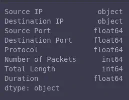
An even more useful field is dtypes, that returns all the data types of the columns in our dataframe:
```
mirai_flow_df.types
```
Pandas Data Types
We can get descriptive statistics, such as count, mean, and standard deviation, with just one function, describe():
```
mirai_flow_df.describe()
```
Pandas Descriptive Statistics

Testing a hypothesis

During data exploration, we often form hypotheses, i.e., assumptions about the data, that we aim to validate as true or false. A commonly used statistical method for this is the t-test, which compares the means of two groups to assess whether they are significantly different.

For instance, suppose we hypothesize that the number of packets per flow in a Mirai packet capture differs significantly from that in a benign packet capture. To test this hypothesis, we use the t-test. The results become even more insightful in scenarios where the data’s origin is unknown (e.g., whether the packet capture is malicious or benign), providing an unbiased perspective on the differences.

The function below demonstrates how to apply the t-test using the ttest_ind package:

from scipy.stats import ttest_ind

def hypothesis_testing(df1, df2, col):
    group1 = df1[col]
    group2 = df2[col]
    pvalue = ttest_ind(group1, group2)[1]
    if pvalue < 0.05:
        return f"The difference between benign and mirai traffic {col} is statistically significant (p < 0.05)"
    else:
        return f"The difference between benign and mirai traffic {col} is not statistically significant (p >= 0.05)"

hypothesis_testing(mirai_flow_df, benign_flow_df, "Number of Packets")

The difference between benign and mirai traffic Number of Packets is statistically significant (p < 0.05)

In this case, we have proven a significant difference between the two packet captures.

Identifying outliers

Outliers are extreme values in a dataset that deviate significantly from the majority of data points. These can often indicate abnormal activity, particularly in network packet captures. One effective method for detecting outliers is by calculating the Z-score.

The Z-score quantifies how far a data point is from the mean, expressed in terms of standard deviations. It is calculated using the formula:

$$ Z = (data\ point - mean\ of\ data\ points) \over standard\ deviation\ of\ data\ points $$

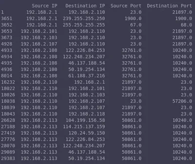
Using this measure, we can identify outliers by determining which values lie significantly far from the average. For example, the zscore function can be used to detect outliers in the total flow length within the Mirai packet capture dataset.

def detect_outliers_zscore(df, column, threshold=3):
    zscores = np.abs(zscore(df[column]))
    return df[zscores > threshold]

outliers = detect_outliers_zscore(mirai_flow_df, "Total Length", threshold=3)
print(outliers)

As demonstrated above, we used a threshold to identify outliers. Specifically, we set a positive threshold, meaning any data point exceeding this value is considered an outlier. In this case, a flow is flagged as an outlier if its total length is more than three standard deviations above the mean. This method is particularly useful for detecting unusually large flows, such as those indicative of file transfers, which can then be investigated further.

Discovering relationships

Correlation and autocorrelation are valuable statistical tools for uncovering relationships between variables. Correlation quantifies the strength and direction (positive or negative) of a linear relationship between two variables. For example, the total number of packets and the total length of a flow are likely to have a positive correlation, as an increase in the number of packets logically results in a longer flow. However, correlations between other variables may be less intuitive.

Converting Data To Numeric Types

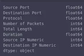
In order to take advantage of the Pandas functions, such as corr, for correlation, we will need to convert our data to numeric types. In the example below, we use ipaddress to convert our IPs to numbers:

import ipaddress

# convert ip address to numeric values
def ip_to_numeric(ip):
    ip_obj = ipaddress.ip_interface(ip)
    return int(ip_obj.network.network_address)

# convert IPs to numeric mirai data
mirai_flow_df["Source IP Numeric"] = mirai_flow_df["Source IP"].apply(ip_to_numeric)
mirai_flow_df["Destination IP Numeric"] = mirai_flow_df["Destination IP"].apply(
    ip_to_numeric
)

Let’s check again our data types to make sure we are ready to calculate the correlation using mirai_flow_df.dtypes:

dtypes2 — Data Types for Mirai traffic after numerical conversions.

Correlation

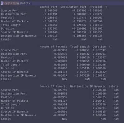
With our data prepared, we can now compute correlations. Below is an example of a correlation matrix generated from the Mirai Pandas DataFrame.

Main Diagonal: The diagonal values represent the correlation of a column with itself (e.g., Source Port correlated with Source Port), which is always equal to 1.
Insights: We observe some significant positive correlations (> 0.5). As expected, there is a strong correlation between Total Length and Number of Packets. Interestingly, we also notice an unexpected correlation between Destination IP and Protocol, which warrants further investigation.

# Calculate the correlation matrix
correlation_matrix = mirai_flow_df.corr()

# Print the correlation matrix and autocorrelation
print("Correlation Matrix:")
print(correlation_matrix)

Autocorrelation measures the similarity between a signal and a delayed version of itself. For example, if the autocorrelation of the Number of Packets is positive and close to 1, this implies a repeating pattern of the number of packets in consecutive time intervals.

# Calculate the autocorrelation for a specific column (e.g., 'Number of Packets')
autocorrelation = mirai_flow_df_numeric['Number of Packets'].autocorr()

print("\nAutocorrelation for 'Number of Packets':")
print(autocorrelation)

This is another demonstration of how useful it is to convert data to Pandas DataFrame and take advantage of its inherent functions.

The cybersecurity perspective

In this blog, we explored statistical methods within the context of cybersecurity, specifically for analyzing network traffic. Below are some key takeaways on the role of statistical EDA in cybersecurity applications:

Hypothesis Testing: In cybersecurity, understanding malicious behavior often involves tackling unknowns since adversaries act unpredictably or attempt to conceal their activities. Developing and testing hypotheses is crucial. For instance, when analyzing software samples with uncertain malware status, you could compare them to known non-malicious samples. A potential hypothesis might be that the size and minimum OS version of a sample are significant indicators of malware. This hypothesis can be tested using statistical methods like the t-test.
Outliers: Outliers—data points that deviate significantly from the norm, often signal abnormal behavior, making them highly valuable in detection engineering. Identifying these outliers, whether visually or statistically, can reveal unusual patterns worth investigating.
Correlation: While “correlation is not causation,” identifying correlations in cybersecurity can uncover meaningful relationships between system characteristics. For example, correlated changes in network traffic patterns might highlight new attack strategies. However, it’s important to avoid over-interpreting correlations. For instance, an observed increase in malicious traffic during colder weather doesn’t imply that lower temperatures cause more network attacks.

Recap

I hope you enjoyed this overview of some interesting statistical methods. While this isn’t an exhaustive list of all possible statistical explorations, it provides a solid starting point. In the next blog, we will dive into data exploration using automation tools, including Python libraries for statistical and visual analysis, as well as Pandas AI.

– Xenia

Going Even Deeper

Code examples for this blog can be found in the notebook blog_eda_2.ipynb.

Statistics

One of my favorite statistics books: Cartoon Guide to Statistics
Masterful visualizations for understanding statistics and probability: Seeing Theory
Oldies but goodies: NIST Handbook of statistical methods
Statistics done wrong ebook

Exploring the data - Statistics